Contents
Background
Gaussian sampling — that is, generating samples from a Gaussian distribution — plays an important role in many cutting-edge fields of data science, such as Gaussian process, variational autoencoder, or generative adversarial network. As a result, you often see functions like tf.random.normal in their tutorials.
But, deep down, how does computer know how to generate Gaussian samples? This series of blog posts will show 3 different ways that we can program our computer (via Python) to do so. You will also see how R and Python generate Gaussian samples using modified versions of some of these methods.
Starting point: the uniform number generator
Of course, we can’t generate Gaussian samples from thin air. Instead, we start with a random number generator that exists in almost all programming languages: the uniform random number generator. It generates a random number that could take any value between 0 and 1. For Python, the numpy.random module uses the Mersenne twister to generate a uniformly-distributed float that is in the interval [0.0, 1.0).
Since Gaussians are better visualized in 2 dimensions — we are all familiar with the Gaussian “blob” in the xy-plane — I will demonstrate the 3 sampling methods in 2-D, especially since one of the methods do generate Gaussians in two dimensions at the same time.

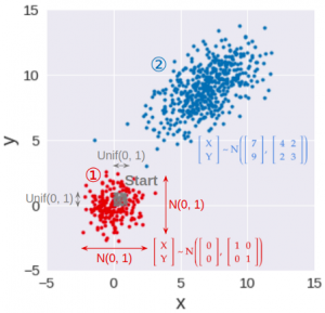
As a result, this series is broken down into 3 parts (see accompanying image):
- The first two parts — part 1 and part 2 — describes 2 common methods to transform the uniform samples (in gray) into points in which their x- and y-coordinates are independent standard Gaussians: both coordinates have a mean of 0, variance of 1, and their covariance is 0 (in red). The first method, the inverse transform sampling, is described below.
- The last part — part 3 — reveals a much simpler alternative to the two methods above in generating standard Gaussian samples. It will also show how to transform these 2-D standard Gaussian samples (in red) to have any given mean or variance in x and y, as well as any given covariance between the x and y coordinates (in blue).
Method 1: Inverse transform sampling
This is the most basic, yet most common, way to convert a uniform random sample into a random sample of any distribution, including Gaussian. This method works by applying the inverse function of the Gaussian CDF (cumulative distribution function) to transform a uniform sample into a Gaussian sample.
To make sure that the Gaussian samples for the x- and y-coordinates are independent, we can use two different uniform samples, one for x (U₁), and one for y (U₂). These two uniform samples can be generated using two different random number generators (two different RandomState initialized by different seeds, for example) so that they are independent in the first place.

How does this work?
This method works by exploiting a mind-blowing principle:
For any distribution, the cumulative probability is always uniformly distributed.
The arithmetic proof of this principle is straightforward but rather boring, and you can view it from this lecture. Instead, I will show the geometric interpretation of this principle. But first, let’s clarify what cumulative probability is: