Background
In part 1 of this project, I’ve shown how to generate Gaussian samples using the common technique of inversion sampling:
- First, we sample from the uniform distribution between 0 and 1 — green points in the below animation. These uniform samples represent the cumulative probabilities of a Gaussian distribution i.e. the area under the distribution to the left of some point.
- Next, we apply the inverse Gaussian cumulative distribution function (CDF) to these uniform samples. This will transform them to our desired Gaussian samples — blue points in the below animation.
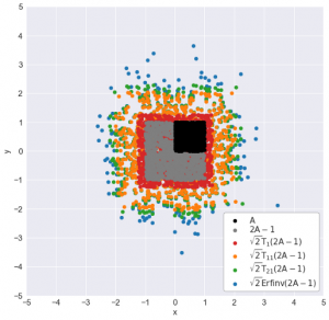
The bad news: the Gaussian inverse CDF is not well-defined, so we have to approximate that function, and the simple Taylor series was used. However, this only samples accurately near the Gaussian mean, and under-samples more extreme values at both ends of the distribution.
Therefore, in this part of the project, we will investigate a more “direct” sampling method that does not depend on the approximation of the Gaussian inverse CDF. This method is called the Box-Muller transform, after the two mathematicians who invented the method in 1958: the British George E. P. Box and the American Mervin E. Muller.

How does the Box-Muller transform work?
For this project, my goal is to generate Gaussian samples in two dimensions i.e. generating samples whose x and y coordinates are independent standard normals (Gaussian with zero mean and standard deviation of 1). In part 1, I used the inverse Gaussian CDF to generate separately the x and y coordinates from their respective uniform samples (U₁ and U₂):
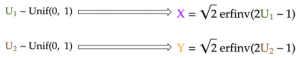
For the Box-Muller transform, I will also start with the same two uniform samples. However, I will transform these uniform samples into the x and y coordinates using much simpler formulas:
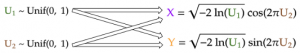
Despite the strong coupling between U₁ and U₂ in each of the two formulas above, the generated x and y coordinates, which are both standard Gaussians, are still surprisingly independent from each other! In the derivation of the Box-Muller transform that follows, I will demonstrate why this is indeed this case.
Derivation of Box-Muller transform
We know that for any two independent random variables x and y, the joint probability density f(x, y) is simply the product of the individual density functions: f(x) and f(y). Furthermore, the Pythagoras theorem allows us to combine the x² and y² terms in each of the Gaussian density functions. This results in the -r²/2 term in the exponential of the joint distribution, where r is the distance from the origin to the 2-D Gaussian sample.

To make it simpler, we then define a variable s that is equal to r²/2. In other words, s is simply half of the squared distance from the origin of our Gaussian sample. Written this way, the joint PDF is simply the product of a constant (1/2π) and an exponential (e⁻ˢ).