Background
The goal of this project is to generate Gaussian samples in 2-D from uniform samples, the latter of which can be readily generated using built-in random number generators in most computer languages.
In part 1 of the project, the inverse transform sampling was used to convert each uniform sample into respective x and y coordinates of our Gaussian samples, which are themselves independent standard normal (having mean of 0 and standard deviation of 1):
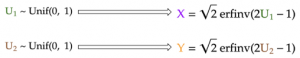
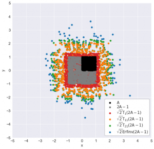
However, this method uses the inverse cumulative distribution function (CDF) of the Gaussian distribution, which is not well-defined. Therefore, we approximated this function using the simple Taylor series. However, this only samples accurately near the Gaussian mean, and under-samples more extreme values at both ends of the distribution.
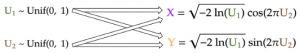
In part 2 of the project, we used the Box-Muller transform, a more direct method to transform the uniform samples into Gaussian ones. The implementation of the algorithm is quite simple, as seen below, but its derivation requires some clever change of variables: instead of sampling Gaussian x and y coordinates for each point, we will sample a uniformly distributed angle (from 0 to 2π) and an exponentially-distributed random variable that represents half of a squared distance of the sample to the origin.
In this part of the project, I will present an even simpler method than the above two methods. Even better, this method is one that every statistics students are already familiar with.
The Central Limit Theorem
It turns out, we can rely on the most fundamental principle of statistics to help us generate Gaussian samples: the central limit theorem. In very simple terms, the central limit theorem states that:
Given n independent random samples from the same distribution, their sum will converge to a Gaussian distribution as n gets large.
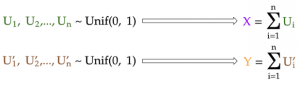
Therefore, to generate a Gaussian sample, we can just generate many independent uniform samples and add them together! We then repeat this routine to generate the next standard Gaussian sample until we get enough samples for our x-coordinates. Finally, we just repeat the same steps to generate the y coordinates.
Note that this method will work even if the samples that we start with are not uniform — they are Poisson-distributed, for example. This is because the central limit theorem holds for virtually all probability distributions *cough let’s not talk about the Cauchy distribution cough*.
Generate Gaussian samples by central limit theorem
To generate, say, 1000 Gaussian sums (n_sums = 1000) where each is the sum of 100 uniform samples (n_additions = 100):
- First, we generate a 100 x 1000 matrix —
uniform_matrix— in which every element is a uniformly distributed sample between 0 and 1. - Then, calculating the 1000 sums is nothing but summing the uniform samples down each column of this matrix, hence the
axis=0argument. The result is a NumPy array ofgaussians, which contains the 1000 Gaussian samples.
n_additions = 100
n_points = 1000# 0. Initialize random number generator
rng = np.random.RandomState(seed=24) # 1. Generate matrix of uniform samples
uniform_matrix = rng.uniform(size=(n_additions, n_points))# 2. Sum uniform elements down each column to get all Gaussian sums
gaussians = uniform_matrix.sum(axis=0)
We can apply the above method to generate Gaussian samples for each coordinate, using different random number generators for x and for y to ensure that the coordinates are independent of each other. Visualizing the intermediate sums after each addition, we see that: