Contents
In a typical Machine Learning project, one would need to find out how good or bad their models are by measuring the models’ performance on a test dataset, using some statistical metrics.
Various performance metrics are used for different problems, depending on what needs to be optimized by the models. For this blog, we will focus on the evaluation metrics that are used in weather forecasting, based on radar images.
The major problem that we need to overcome in our forecasting model is to quickly, precisely, and accurately predict the movement of rain clouds in a short period. If heavy rain is predicted as showers or – even worse – as cloudy weather without rain, the consequences could be serious for the users of our prediction model. If the rain is going to stop in the next few minutes, incorrect forecasting – that predicts that rainfall would continue with high intensity – may cause little to no harm; however, the prediction model is no longer useful.
A good model should tackle as many of these issues as possible. We believe that the following measures may help us identify which model is better.
Performance Metrics
- Root Mean Square Error (RMSE): This is a broad measure of accuracy in terms of an average error across the value of forecast-observation pairs. Formally, it is defined as follows:
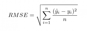 This measure will help us to compare how much difference intensity between ground truth observation and predicted one.
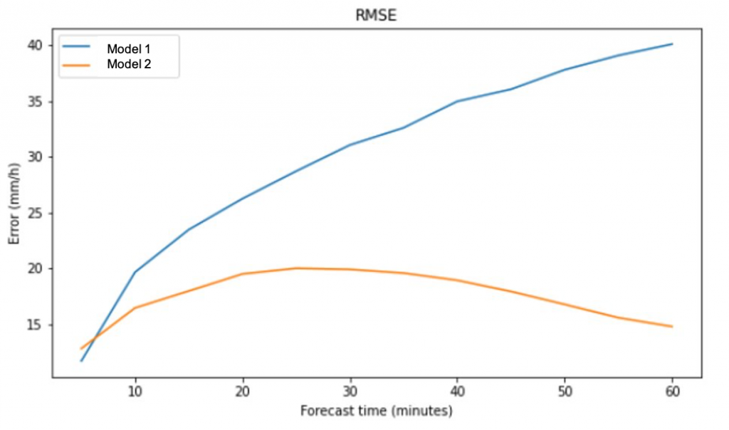 Figure 1: RMSE between 2 models across 60 minutes forecast.
Figure 1 shows an example of the RMSE between 2 different models over 60 minutes forecast.
The RMSE of Model 1 is increasing over time. On the other hand, it seems that Model 2 has a smaller RMSE, which means it is a better model out of the two models.
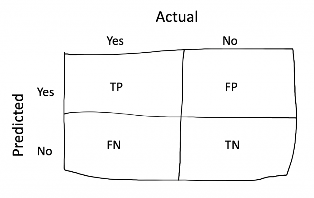
Before defining the next metric, we need to recall about Confusion Matrix (Figure 2). Each column of the matrix represents the instances in an actual class while each row represents the instances in a predicted class, or vice versa [1]. By using Confusion Matrix, we can calculate the number of False Positives (FP), False Negatives (FN), True Positives (TP), and True Negatives (TN).
- Hit Rate (H): The fraction of observed events that are forecast correctly. This is also known as the Probability of Detection. It tells us what proportion had rain was predicted by the algorithm as having rain. It ranges from [0,1].
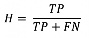
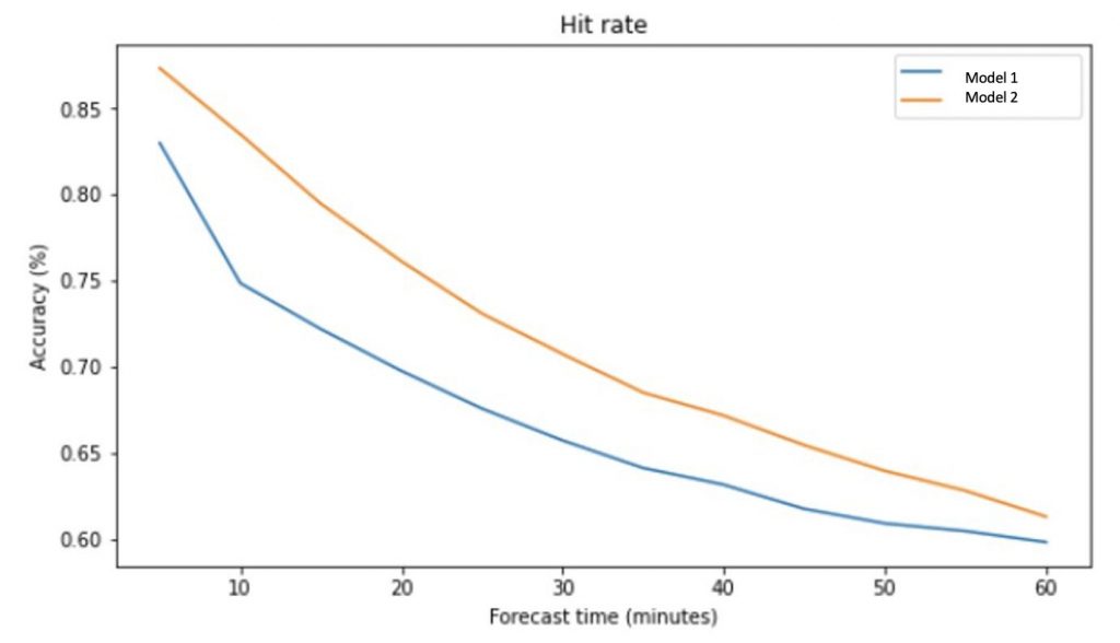
Figure 3: Hit rate of 2 models across 60 forecast times.
From Figure 3, the Hit Rate of both models is good in the first 20 minutes. Model 2 has a higher value than model 1 (higher probability of predicting rain). Therefore, model 2 is the better model base on this measure.
- False Alarm Ratio (FAR): The fraction of “yes” forecasts that were wrong. It is calculated as follows:
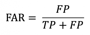
Even though in weather forecast the False Alarms do not lead to serious consequences. However, a model with a high FAR measure is not ideal.
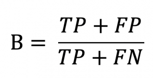
- Bias (B): This measure compares the number of points is predicted as having rain and the total number of actual rain points. Specifically,