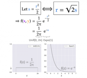
This is where it gets interesting since we can think of the 1/2π constant as a uniform distribution between 0 and 2π: Unif(0, 2π). On the other hand, the exponential term is nothing but an exponential distribution with the parameter λ=1: Expo(1). Furthermore, since these two terms are multiplied together in the joint distribution, the uniform and the exponential distributions are also independent of each other (see accompanying image).

Geometric interpretation

 

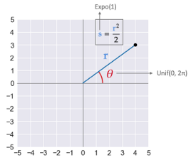
Geometrically, the uniform distribution between 0 and 2π represents the angle θ that our 2-D Gaussian sample makes with the positive x-axis. This aligns with our intuition about Gaussian samples in 2-D: they are sampled with an equal chance at any angle between 0 and 360 degrees, hence the characteristic round “blob” that they often make.

In contrast, these blobs are always concentrated near the origin, which fits well with the fact that s (half of the squared distance from the origin) follows an exponential distribution: you are more likely to encounter a sample as you move closer to the origin.

This leads us to the underlying principle of the Box-Muller transform:

Instead of sampling independent Gaussians for the x and y coordinates of the samples, we sample their independent uniform angles and exponential half-of-squared distances to origin.

Caveat for changing variables

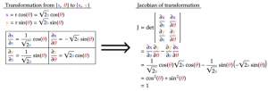
Technically, when changing random variables of a joint distribution to different ones, we need to multiply the new distribution with the Jacobian of the variable transformation (see here for more details). This ensures that the new distribution is still a valid probability density function i.e. that the “area” under the distribution is still 1. Thankfully, the Jacobian of the transformation from {s, θ} to {x, y} is 1, which greatly simplifies our problem.

 

Sampling 2-D Gaussians with Box-Muller transform

Once we transform the original problem into sampling a uniform angle and an exponential half-of-squared-distance, the remaining steps are much easier. This is because both the uniform and the exponential distribution have very simple inverse CDF, as outlined in the table below. As a result, we can apply these inverse CDFs to any uniform sample from 0 to 1 to transform it to our desired uniform and exponential sample (see part 1 of the project for an explanation of inverse transform sampling).

 

The animation below walks through all the steps needed to generate the Gaussian samples in 2-D:

1. Sample from two separate uniform sample generators (U₁ and U₂)
2. Apply the inverse CDF of the exponential distribution with λ=1 to U₁ to get half of the squared distance from the origin of the sample (s). For simplicity, the inverse CDF is modified from -ln(1-U₁) to -ln(U₁). As a result, this modified function is technically no longer the inverse CDF of the exponential, but it will still output samples that are exponentially distributed. This is because U₁ and 1-U₁ are both uniform samples between 0 and 1.
3. Apply the inverse CDF of the uniform distribution between 0 and 2π to U₂ to get the angle of the sample (θ)
4. Calculate the distance r from the origin for each sample from its half of squared distance: r=√(2s).
5. Lastly, the x and y coordinates are found by simple trigonometry: r cos(θ) and r sin(θ) respectively. Combining the formulas from steps 2 to 5 gives us the formulas seen earlier to transform U₁ and U₂ into x and y.

Coding-wise, generating Gaussian samples using the Box-Muller transform can’t be any easier, as seen in this Python implementation for the 5 steps mentioned above to generate 1000 Gaussian samples in 2-D:

For more detail, please check the Link

Please also check N-gram language models and Bayesian Statistics.