In any data science project, once the variables that correspond to business objectives are defined, typically the project proceeds with the following aims: (1) to understand the data quantitatively, (2) to describe the data by producing a ‘model’ that represents adequately the data at hand, and (3) to use this model to predict the outcome of those variables from ‘future’ observed data.

Anyone dealing with machine learning is bound to be familiar with the phenomenon of overfitting, one of the first things taught to students, and probably one of the problems that will continue to shadow us in any data-centric job: when the predictive model works very well in the lab, but behaves poorly when deployed in the real world.

What is Overfitting?

Overfitting is defined as “the production of an analysis which corresponds too closely or exactly to a particular set of data, and may therefore fail to fit additional data or predict future observations reliably.”

Whether a regression, decision tree, or neural network, the different models are constructed differently: some depend on a few features (in the case of a linear model), some are too complex to visualize and understand at a glance (in the case of a deep neural network). Since there is inherently noise in data, the model fitting (‘learning’) process can either learn too little pattern (‘underfit’) or learn too many ‘false’ patterns discernible in the ‘noise’ of the seen data (‘overfit’) not meant to be present in the intended application, that end up distorting the model. Typically, this can be illustrated in the diagram below:

Detecting overfitting

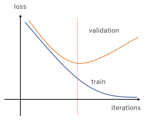
In Machine Learning (ML), training and testing are often done on different parts of data available. The models — whether they be trees, neural networks, equations — that have characterized the training data very well, are validated on a ‘different’ part of data. Overfitting is detected when the model has learned too many ‘false patterns’ from the training data that do not generalize to the validation data. As such, most ML practitioners reduce the problem of overfitting to a matter of knowing when to stop training, typically by choosing an ‘early stopping’ value around the red dotted line, illustrated in the loss vs. several iterations graph below.

If detecting overfitting is reduced to a matter of “learning enough”, inherent to the contemporary ML training process, it is assumed to be “solved” when the model works on a portion of the held-out data. In some cases, k-fold / cross-validation is performed, which splits the data into k ‘folds’: one held-out test set and k-1 training sets. Given that most models do not make it to the crucible of the production environment, most practitioners stop at demonstrating (in a lab-controlled environment) that the model “works”; when the numbers from cross-validation statistics check out fine, showing consistent performance across all folds.

But.. is it so simple?

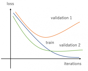
In simpler or more trivial models, overfitting may not even be noticeable! However, with more rigorous testing or when the model is lucky enough to be deployed to the production stage, there is usually more than one validation set (or more than one client’s data!). It is not infrequent that we see various validation/real-world data do not ‘converge’ at the same rate, making the task of choosing an early stopping point more challenging. With just two different validation data sets, one can observe the following:

What about this curve?

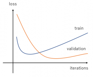
When we get curves that look like the graphs above, it is harder to answer these questions: When does overfitting ‘begin’? How to deal with multiple loss functions? What is happening here??

Digging your way out

Textbook ML prescribes many ‘solutions’ — which might just work if you are lucky — sometimes without you knowing exactly what is the problem:

• Data augmentation:

  Deep down, most overfitting problems will go away if we have an abundant amount of ‘good enough’ data, which for most data scientists is a utopian dream. Limited resource makes it impossible to collect the perfect data: clean, complete, unbiased, independent, and cheap. For many neural network ML pipelines, data augmentation has become de rigeur, which aims to make the model not learn characteristics unique to the dataset, by multiplying the amount of training data available. Without collecting more data, data can be ‘multiplied’ by varying them through small perturbations to make them seem different from the model. Whether or not this approach is effective will depend on what is your model learning!

• Regularization:

  The regularization term is routinely added in model fitting, to penalize overly complex models. In regression methods, L1 or L2 penalty terms are often added to encourage smaller coefficients and thus, ‘simpler’ models. In the decision trees, methods such as decision tree pruning or limiting tree maximum depth, are typical ways to ‘keep model simple’. Combined with ensemble methods, e.g. bagging or boosting, they can be used to avoid overfitting and make use of multiple weak learners to arrive  at a robust predictor. In DL techniques, regularization is achieved by introducing a dropout layer, that will randomly turn off neurons during training.

If you have gone through all those steps outlined above and still feel somehow that you just got lucky with a particular training/validation data set, you are not alone. We need to dig deeper to truly understand what is happening and get out of this sticky mess, or accept the risk of deploying such limited models and set up a future trap for ourselves!