Contents
On a nice day 2 years ago, when I was in the financial field. My boss sent our team an email. In this email, he would like to us propose some machine learning techniques to predict stock price.
So, after accepting the assignment from my manager, our team begin to research and apply some approaches for prediction. When we talk about Machine Learning, we often think of supervised and unsupervised learning. But one of the algorithms we applied is one that we forgot however equally highly effective algorithm: Monte Carlo Simulation.
What is Monte Carlo simulation?
The Monte Carlo method is a technique that uses random numbers and probability to solve complex problems. The Monte Carlo simulation, or probability simulation, is a technique used to understand the impact of risk and uncertainty in financial sectors, project management, costs, and other forecasting machine learning models.[1]
Now let’s jump into python implementation to see how it applies,
Python Implementation
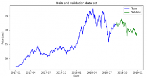
In this task, we used data of DXG stock dataset from 2017/01/01 to 2018/08/24 and we would like to know what is stock price after 10 days, 1 month, and 3 months, respectively
We will simulate the return of stock and next price will be calculated by
P(t) = P(0) * (1+return_simulate(t))
Calculate mean and standard deviation of stock returns
miu = np.mean(stock_returns, axis=0)
dev = np.std(stock_returns)
Simulation process
simulation_df = pd.DataFrame()
last_price = init_price
for x in range(mc_rep):
    count = 0
    daily_vol = dev
    price_series = []
    price = last_price * (1 + np.random.normal(miu, daily_vol))
    price_series.append(price)
    for y in range(train_days):
        if count == train_days-1:
            break
        price = price_series[count] * (1 + np.random.normal(miu, daily_vol))
        price_series.append(price)
        count += 1
    simulation_df[x] = price_series
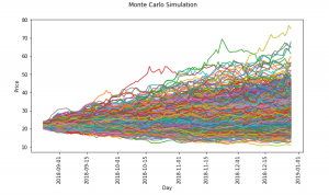
Visualization Monte Carlo Simulation
fig = plt.figure()
fig.suptitle('Monte Carlo Simulation')
plt.plot(simulation_df)
plt.axhline(y = last_price, color = 'r', linestyle = '-')
plt.xlabel('Day')
plt.ylabel('Price')
plt.show()
Now, let’s check with actual stock price after 10 days, 1 month and 3 months
plt.hist(simulation_df.iloc[9,:],bins=15,label ='histogram')
plt.axvline(x = test_simulate.iloc[10], color = 'r', linestyle = '-',label ='Price at 10th')
plt.legend()
plt.title('Histogram simulation and last price of 10th day')
plt.show()
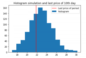
We can see the most frequent occurrence price is pretty close to the actual price after 10th
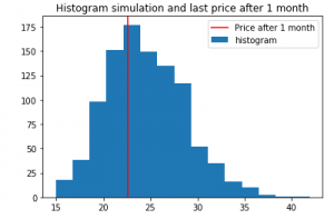
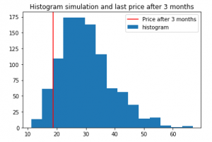
If the forecast period is longer, the results are not good gradually
Simulation for next 1 month
After 3 months
Conclusion
Monte Carlo simulation is used a lot in finance, although it has some weaknesses, hopefully through this article, you will have a new look at the simulation application for forecasting.
Reference
[1] Pratik Shukla, Roberto Iriondo, “Monte Carlo Simulation An In-depth Tutorial with Python”, medium, https://medium.com/towards-artificial-intelligence/monte-carlo-simulation-an-in-depth-tutorial-with-python-bcf6eb7856c8Please also check Gaussian Samples and N-gram language models,
Bayesian Statistics for more statistics knowledge.
Hiring Data Scientist / Engineer
We are looking for Data Scientist and Engineer.
Please check our Career Page.
Data Science Project
Please check about experiences for Data Science Project
Vietnam AI / Data Science Lab

Please also visit Vietnam AI Lab