Contents
- The 2-D samples start confined in a length-one block near the origin since their coordinates all began as uniform samples between 0 and 1. However, as more and more samples are added on top of each uniform sample, they start to “grow” toward the familiar Gaussian blob in the xy-plane.
- This is also reflected in the histogram of the sampled x and y coordinates: they start as single peaks that represent the Unif(0, 1) distribution. As more samples are added, they level out towards the familiar bell curve of the Gaussian distribution.
- Lastly, the QQ-plot of the samples first followed the S-shaped pattern of lighter-tailed distributions, which include the uniform. Then, it quickly conforms to the diagonal line, even when only 10 samples have been added. In other words, adding even just a few uniform samples already gives us sums that are characteristically Gaussian.
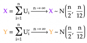
In short, the central limit theorem allows us to easily generate Gaussian samples in 2-D, whose x and y coordinates are the Gaussian sums of many uniform samples. However, we still need to rescale these x and y coordinates so that they return to standard normal (mean of 0 and standard deviation of 1).
Rescale Gaussian samples
Rescaling the Gaussian samples means we have to subtract each sum by its mean and divide by its standard deviation.
- For a sum of n uniform samples, the mean of the sum is simply the sum of all the uniform means, which are 1/2 each. Therefore, the mean of the generated Gaussian sample is n/2.
- Furthermore, since these uniform samples are independent, the variance of their sum is simply the sum of the uniform variances, which are 1/12 each. Hence, the variance of the generated Gaussian sample is n/12, and its standard deviation is √(n/12).

As a result, the Gaussian samples that represent the x and y coordinates can be normalized as follows:
Please check more detail in the Link
Please also check N-gram language models and Bayesian Statistics.
Data Science Blog
Please check our other Data Science Blog
